Pipeline Examples & Results
Real-world example showing the complete pipeline workflow with actual data
Example Dataset Overview
This example demonstrates a complete pipeline run from January 13, 2026
Data Collection
- • Grid size: 5×5 points (0.0 to 0.2m in both X and Y)
- • Total measurements: 50 points
- • Measurement spacing: 0.05m intervals
- • Coverage area: 0.2m × 0.2m
Data Quality
- • Valid measurements: 50 (100%)
- • Flagged points: 3 (6%)
- • Final clean data: 47 points
- • Sample rate: 0.303 Hz
Pipeline Steps with Example Data
Raw Data Collection (mag_to_csv.py)
Initial sensor measurements from MMC5983MA magnetometer
Data Structure
The raw data contains timestamped measurements with spatial coordinates (x, y) and magnetic field components (Bx, By, Bz) along with computed B_total.
time,x,y,Bx,By,Bz,B_total,units
2026-01-13T19:52:50.143+00:00,0.0,0.0,4.328137817382813,0.2996209716796875,0.7353729248046875,4.400377601009411,gauss
2026-01-13T19:52:53.462+00:00,0.05,0.0,0.01,-0.018399658203125,-0.106656494140625,0.10869293980917528,gauss
2026-01-13T19:52:56.630+00:00,0.1,0.0,0.0124932861328125,0.006651611328125,-0.07955078125,0.08080008000702794,gauss
2026-01-13T19:52:59.675+00:00,0.15000000000000002,0.0,0.0114398193359375,0.00701171875,-0.0683447265625,0.06964937411901764,gauss
2026-01-13T19:53:02.631+00:00,0.2,0.0,0.006602783203125,0.0071014404296875,-0.076580810546875,0.07719227776287102,gauss
2026-01-13T19:53:05.735+00:00,0.0,0.05,0.008687744140625,-0.0266925048828125,-0.0593548583984375,0.06565794643963897,gauss
...Validated & Cleaned Data (validate_and_diagnosticsV1.py)
Data after validation, outlier detection, and spike detection
Quality Flags Added
The validation script adds three flag columns to identify problematic data points:
- •
_flag_outlier: 3 points with extreme B_total values - •
_flag_spike: Points with sudden jumps between consecutive measurements - •
_flag_any: Combined flag (outlier OR spike)
time,x,y,Bx,By,Bz,B_total,units,_time_utc,_flag_outlier,_flag_spike,_flag_any
2026-01-13T19:52:53.462+00:00,0.05,0.0,0.01,-0.018399658203125,-0.106656494140625,0.1086929398091752,gauss,2026-01-13 19:52:53.462000+00:00,False,False,False
2026-01-13T19:52:56.630+00:00,0.1,0.0,0.0124932861328125,0.006651611328125,-0.07955078125,0.0808000800070279,gauss,2026-01-13 19:52:56.630000+00:00,False,False,False
2026-01-13T19:52:59.675+00:00,0.15,0.0,0.0114398193359375,0.00701171875,-0.0683447265625,0.0696493741190176,gauss,2026-01-13 19:52:59.675000+00:00,False,False,False
...
Validation Statistics
B_total Statistics
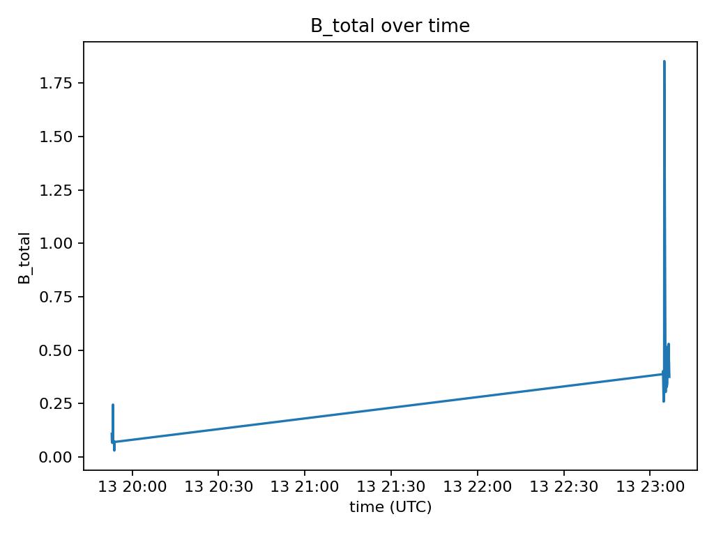
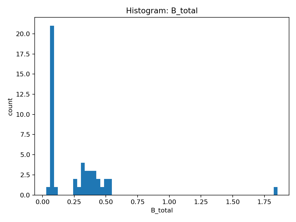
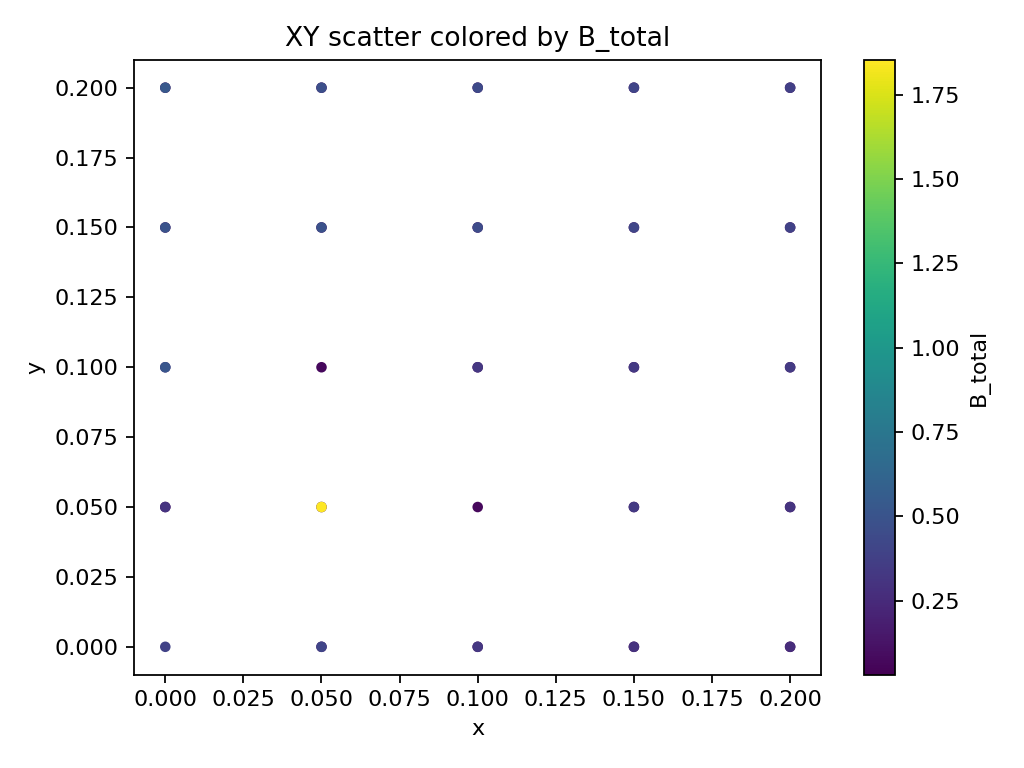
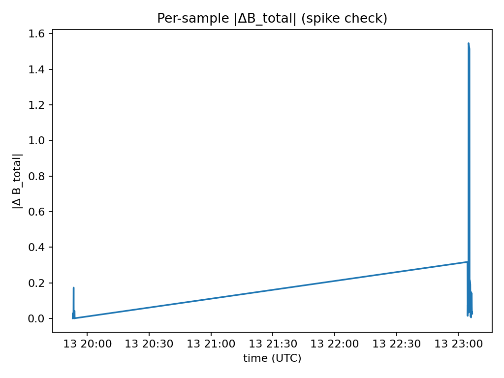
Diagnostic Plots Generated
The validation script automatically generates several diagnostic visualizations:
- • B_total vs time - Time series showing magnetic field over measurement period
- • Histogram of B_total - Distribution of magnetic field values
- • XY scatter plot colored by B_total - Spatial distribution of measurements
- • Spike deltas plot - Identification of sudden changes between measurements
B_total over time
Histogram of B_total
XY scatter plot colored by B_total
Per-sample |ΔB_total| (spike check)
Anomaly Detection (compute_local_anomaly_v2.py)
Local anomaly computation comparing each point to its neighborhood
Anomaly Columns Added
The anomaly detection script adds three new columns to the cleaned data:
- •
local_anomaly: Raw anomaly value (B_total - local_mean) - •
local_anomaly_abs: Absolute value of the anomaly - •
local_anomaly_norm: Normalized anomaly (0-1 scale)
time,x,y,Bx,By,Bz,B_total,units,_time_utc,_flag_outlier,_flag_spike,_flag_any,local_anomaly,local_anomaly_abs,local_anomaly_norm
2026-01-13T19:52:53.462+00:00,0.05,0.0,0.01,-0.018399658203125,-0.106656494140625,0.1086929398091752,gauss,2026-01-13 19:52:53.462000+00:00,False,False,False,-0.2185578102616949,0.2185578102616949,-0.13485824132575147
2026-01-13T19:52:56.630+00:00,0.1,0.0,0.0124932861328125,0.006651611328125,-0.07955078125,0.0808000800070279,gauss,2026-01-13 19:52:56.630000+00:00,False,False,False,-0.23376565643511524,0.23376565643511524,-0.14424204411387573
...
Key Insight
In this example dataset, one point at (0.05, 0.05) shows a significant positive anomaly with a local_anomaly value of 1.62 gauss and a normalized value of 1.0 (maximum). This indicates a strong local magnetic disturbance compared to surrounding measurements, which could indicate a structural anomaly, rebar concentration, or other subsurface feature.
Heatmap Visualization (interpolate_to_heatmapV1.py)
IDW interpolation and heatmap generation
Output Files
- •
mag_data_grid.csv: Regular grid with interpolated local_anomaly values - •
mag_data_heatmap.png: Visual heatmap showing spatial distribution of anomalies
Heatmap Interpretation
The heatmap visualizes the spatial distribution of local magnetic anomalies using a color gradient:
- • Yellow/Red regions: High positive anomalies (stronger magnetic field than neighbors)
- • Green regions: Neutral anomalies (similar to neighborhood average)
- • Blue/Purple regions: Low negative anomalies (weaker magnetic field than neighbors)
Heatmap (IDW) of local_anomaly
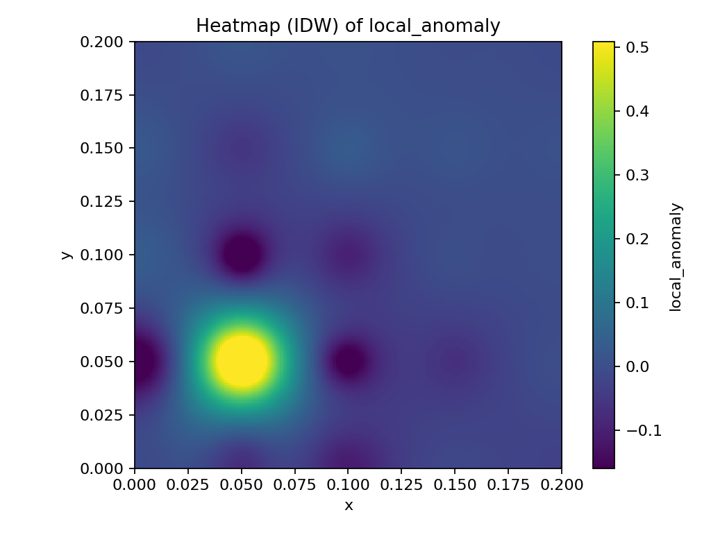
The heatmap shows distinct anomaly patterns with several hotspots (yellow) and coldspots (blue/purple) distributed across the measurement grid.
Complete Workflow Summary
Data Collection
Collected 50 measurements across a 0.2m × 0.2m grid using auto-grid mode.
Validation & Cleaning
Identified and flagged 3 problematic points (6%), resulting in 47 clean data points ready for analysis.
Anomaly Detection
Computed local anomalies for all 47 points, identifying significant magnetic disturbances including a major anomaly at (0.05, 0.05) with normalized value of 1.0.
Visualization
Generated interpolated grid and heatmap visualization showing spatial distribution of anomalies, ready for interpretation and further analysis.